Cette page était sur le site de
PY4ZBZ; mais le lien ayant disparu, j'ai reproduit ici l'article
que j'avais conservé. (F5AD)
********************************
THE SECRETS OF THE LOG PERIODIC ANTENNA
Lightweight
and precise, the log periodic has become
a favorite among EMC engineers.
JON CURTIS AND ISIDOR STRAUS,
CURTIS-STRAUS, LLC (978)
486-8880
In 1957, at precisely the same time that Wilmar Roberts was developing his famous precision dipoles for the FCC, R.H. DuHamel and D.E. Isbell published the first work on what was to become known as log periodic arrays. Their remarkable antennas exhibited relatively uniform input impedances, VSWR, and radiation characteristics over a wide range of frequencies. The design was so simple that in retrospect it is remarkable that it took so many years for someone to happen upon it. Log periodic array are, after all, simply a group of dipole antennas strung together and fed alternately through a common transmission line. Still, despite its simplicity, the log periodic antenna remain a subject of considerable study. Only recently was it realized that the log periodic was one of a class of antennas known as fractal antennas which are now at the cutting edge of antenna development.
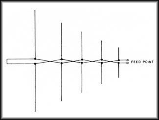
The log periodic antenna works the way one intuitively would expect. Its active region, that portion of the antenna which is actually radiating or receiving radiation efficiently, shifts with frequency. The left most element in Figure 1 (the longest element) is active at the lowest frequency of interest where it acts as a half wave dipole. As the frequency shifts upward, the active region shifts forward. The upper frequency limit of the antenna is a function of the right most, or shortest, element.
Log periodic designs have been proposed in a variety of geometries, but the one most commonly used for EMC work is the Log Periodic Dipole Array (LPDA) of Figure 1 invented by D.E. Isbell of the University of Illinois. The LPDA we’ll discuss in this article covers a frequency range of 200 to 1000 MHz. We didn’t build it, but we did simulate its operation on a Method of Moments simulator.
Figure 1: Basic arrangement
of a Log Periodic Dipole
Array (LPDA) From Ref. 1.
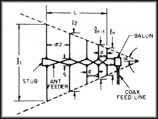
Figure 2: A closer look at
the LPDA. Note that adjacent
elements are fed out of phase.
Figures 1 and 2 describe the
basic geometry. Each element is shorter than the element to its
left. Ratio of each element to each adjacent element is constant,
and is given a value known as tau (![]() ). The
other critical dimension is the spacing between elements
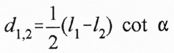
designated "d" in Figure 2. Distance d1,2
for example, is the distance between the left most element and
its nearest neighbor. The distance between two adjacent elements
is:
). The
other critical dimension is the spacing between elements
designated "d" in Figure 2. Distance d1,2
for example, is the distance between the left most element and
its nearest neighbor. The distance between two adjacent elements
is:
The two
factors, tau (![]() ) and
sigma (
) and
sigma (![]() ),
are pretty much the only factors we have to consider in designing
our array. Tau is the ratio of the length of one element to its
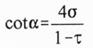
next longest neighbor. Sigma is known as the "relative
spacing constant" and along with determines the angle of the
antenna’s apex, alpha (a).
),
are pretty much the only factors we have to consider in designing
our array. Tau is the ratio of the length of one element to its
next longest neighbor. Sigma is known as the "relative
spacing constant" and along with determines the angle of the
antenna’s apex, alpha (a).
Tau and sigma can be selected by using Figure 3 [Ref. 1, 3]. For EMC work, we’d like to keep the antenna as compact as possible, and we can do so by selecting a low tau. We also would like to keep the gain fairly low so as to avoid too narrow a beam width. We’ll choose a sigma of .12 and a tau of .8, which should produce an antenna with a gain of approximately 6.5 db over isotropic.
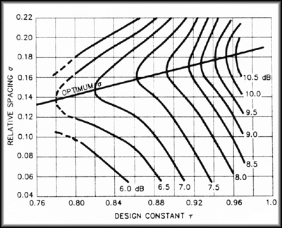
Figure 3: The parameters
tau and sigma can be chosen from this graph.
We chose a tau of .8 and a sigma of .12 for a predicted gain of
6.5 dBi.
The line for optimum sigma is for those designers who want
maximum
gain. [Ref. 1, 3].
In operation, the LPDA works as follows. Figure 2 illustrates an LPDA with five elements [after Ref. 1]. Assume that we are operating on a frequency in which the third (middle) element is resonant. Elements 2 and 4 are slightly longer and shorter, respectively, than element 3. Their spacing, combined with the fact that the transmission line flips 180 degrees in phase between elements allows these two elements to be in phase and nearly (but not quite) resonant with element 3. Element 4, being slightly shorter that element 3 acts as a "director" shifting the radiation pattern slightly forward. Element 2, being slightly longer acts as a "reflector" further shifting the pattern forward. The net result is an antenna with gain over a simple dipole. As the frequency shifts, the active region, those elements which are receiving or transmitting most of the power, shifts along the array.
Having chosen tau and sigma, we simply plug in the numbers. The result is Table 1.
| The
antenna is fed through a 200:50 ohm balun. Tau = .8 Sigma = .12. Gain = 6.5 dBi. Alpha = 22.6 degrees. Cot a = 2.4 l1 = 492/(200 Mhz) = 2.46 feet = 29.52 inches. lmin = 492/(1000 Mhz) = .492 feet = 5.9 inches. |
||
| Element | Formula |
Length (inches) |
| l1 | (492/200) ft. | 29.52 |
| l2 | l1
|
23.64 |
| l3 | l2
|
18.84 |
| l4 | l3
|
15.11 |
| l5 | l4
|
12.09 |
| l6 | l5
|
9.67 |
| l7 | l6
|
7.74 |
| l8 | l7
|
6.19 |
| l9 | l8
|
4.95 |
| Spacing Between Elements | Formula | Distance (inches) |
| d1,2 | .5(l1 - l2) cot a | 7.08 |
| d2,3 | d1,2
|
5.64 |
| d3,4 | d2,3
|
4.56 |
| d4,5 | d3,4
|
3.60 |
| d5,6 | d4,5
|
2.88 |
| d6,7 | d5,6
|
2.28 |
| d7,8 | d6,7
|
1.86 |
| d8,9 | d7,8
|
1.49 |
Now comes the tricky part. We have to select the characteristic impedance of the transmission line that feeds the elements, a transmission line which, in our case, also acts as the boom of the antenna. We will call this transmission line impedance Zb (for boom) and Ref. 1 tells us it should be:
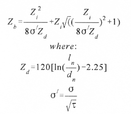
Equation 3 deserves some explanation. Zd is the characteristic impedance of a simple dipole antenna. As stated previously, Zb is the characteristic impedance of the boom, itself a transmission line (referred to as the antenna feeder line in Figure 2). Zi is the impedance of the antenna as seen from its input terminals. Those terminals are usually connected to some kind of balun which performs the balanced to unbalanced transformation and steps down the impedance Zi to match the impedance of the line running between the antenna and the signal source (when transmitting) or receiver input (when receiving). The impedance is of this line, referred to as the coax feed line in Figure 2, is usually 50 ohms and we will refer to it as Z0.
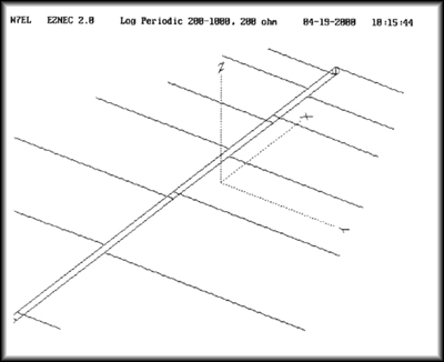
Figure 4: The antenna
we have chosen to model uses two booms acting as a
transmission line feeding the antenna elements.
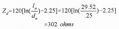
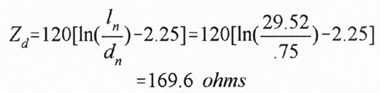
We have chosen to make the antenna elements from 1/4 inch rods. That makes the impedance Zd of the longest element:
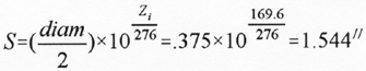
Next we choose the spacing between the two booms which make up the transmission line feeding the elements. We’ll choose a style for the log periodic antenna shown in Figure 4. The two booms consist of one quarter inch rods to which the left and right elements are alternately attached. Note that each element making up the antenna is fed 180 degrees out of phase with the elements adjacent to it. For reasons that will become apparent shortly, we will need to choose a relatively high impedance to feed the booms (Z i ). We’ll choose 200 ohms. This impedance is four times the characteristic impedance of our coaxial line (Z0 = 50 ohms) and is readily produced through the use of a balun with a 2:1 ratio of windings. The spacing between the two booms then becomes [after Ref. 1]:
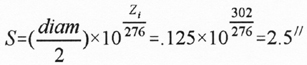
Where:
diam = diameter of each boom in
inches.
S = center to center spacing between the booms in inches.
We won’t be able to hold each element’s ratio of the length to the diameter constant since metal stock isn’t available in all sizes. We’ll choose diameters which attempt to preserve a length to diameter ratio of approximately 118 (Table 3).
The last design element we will have to calculate is the terminating stub shown in Figure 1. After Ref. 1, this is set at max / 8 or 7.4."
It now remains to plug in these numbers to a Methods of Moments program. We’ll choose EZNEC, being mindful of some the limitations of the Methods of Moments technique. Log periodic antennas can be particularly challenging to model. Through the use of a "Guidelines Check" built into the software, allegiance to the limitations in Table 2 can be automatically checked. We end up with the choice of parameters for each element shown in Table 3 and then press enter to start the simulation.
Can You Always Trust MOM? EZNEC warns us to observe the following
limitations, least it produce
Diameters of all wires should be <
.02
Use at least 20 segments per each half wavelength.
Wire spacing should be > .0015
Transmission line spacings should be greater than several wire diameters.
Voltage sources feeding transmission
lines should be on a wire 3 segments long and > .02
At their connection point, the ratio of any two wire diameters should be < 2:1. |
Table 2
The predicted VSWR for the antenna over a frequency range 200 to 1000 MHz is shown in Figure 5(a). The VSWR is quite good except above 700 MHz. We can make a reasonable guess that the problem at the high end is due to the shortest elements being to long, and so we trim .5 inch off these and run the simulation again. Now the VSWR barely rises above the 1.5:1 range.
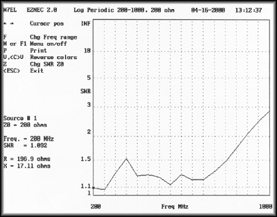
Figure 5a
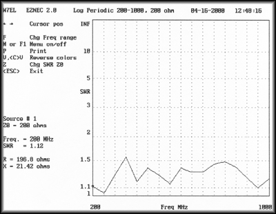
Figure 5b
Figure 5:
Figure 5a shows the predicted VSWR fpr the antenna described in
Tables 1 and 3.
Shortening the two elements that make up the
shortest elements of the array by .5 inch each
yields the VSWR plot of Figure 5b
The radiation patterns and gain over isotropic at 200, 500, 700 and 1000 MHz are shown both as "elevation" and "azimuth" patterns in Figure 6. The elevation pattern is the field produced in a plane that slices through the boom of the antenna and is perpendicular to the antenna elements. The azimuth pattern is the field strength in the plane that the antenna elements lie in. Both show the expected forward gain which varies from 5 dBi to 7 dBi, reasonably close to our design target of 6.5 dBi.
Our antenna can now be built and should perform well. One drawback to the design, though, is the 200:50 balun that has to be used. Such baluns can introduce losses and may have difficulty in handling the high powers that are sometimes used for susceptibility testing. For this reason, some commercial design aim at setting the characteristic impedance of the boom at something close to 50 ohms, 75 ohms being a typical target. (Setting the impedance of the boom elements at 50 ohms is not possible when round booms are in use.)
To get such a low impedance, we will have to use thick booms and antenna elements. For the purposes of our example, we will choose .75 inch diameter pipe. First we compute Z d for .75: inch elements:
Then we can calculate the boom center to center spacing:
Unfortunately, this log periodic antenna will have to be built to be tested. Its large size elements and close spacings (.044" between the booms) will cause it to exceed the parameters of Table 2. Yes, even in the 21st century there are some things best left to craftspersons, not computers.
Those craftspersons know a few other tricks. One is to dispense with the 50:75 ohm balun and just suffer with a slightly higher VSWR. In order to allow for a balanced to unbalanced transformation, ferrite beads can be slipped over the 50 ohm coaxial cable, producing what’s known as a W2DU balun [Ref. 1].
Log periodic antennas are rugged, simple and versatile. They will remain one of the best tools available to the EMC engineer for years to come.
References
1. The ARRL Antenna Book, The American Radio Relay League, Newington, CT, 1991.
2. R. H. DuHamel and D. E. Isbell, "Broadband Logarithmically Periodic Antenna Structures," 1957 IRE National Convention Record, Part 1.
3. R. L. Carrell, "The Design of Log-Periodic Dipole Antennas," 1961 IRE International Convention Record, Part 1.
Copyright and Disclaimer
©2000
Conformity®